Introduction to AI and Machine Learning Landscape
The realm of Artificial Intelligence (AI) and Machine Learning (ML) is a rapidly evolving universe, characterized by the continuous emergence of revolutionary paradigms, algorithms, and methodologies aimed at solving complex problems and enhancing the capabilities of machines to learn from and interpret data. At the heart of this transformative journey are the two formidable pillars of machine learning models: Recurrent Neural Networks (RNNs) and Transformers. Both architectures have been instrumental in propelling advancements in fields such as natural language processing (NLP), computer vision, and time-series forecasting. However, as we delve deeper into the nuances of each, it becomes evident that their operational principles, strengths, and limitations diverge considerably, shaping the future trajectory of AI development and application.
The Evolutionary Path of RNNs
Recurrent Neural Networks, or RNNs, are a class of neural networks that excel in handling sequences of data, making them particularly suited for tasks that involve temporal dependencies, such as language translation, voice recognition, and financial forecasting. RNNs are designed to remember the output of a node and feed this back into the network as input, creating a form of memory that allows them to maintain context across time steps.
However, RNNs are not without their shortcomings. They are notoriously difficult to train due to problems like vanishing and exploding gradients, which inhibit the model’s ability to learn long-range dependencies. These challenges have led researchers and developers to explore alternative architectures and improvements, such as Long Short-Term Memory (LSTM) networks and Gated Recurrent Units (GRUs), both of which introduce mechanisms to better control the flow of information and mitigate the aforementioned issues.
# Example of a simple RNN model in TensorFlow from tensorflow.keras.models import Sequential from tensorflow.keras.layers import SimpleRNN, Embedding, Dense model = Sequential() model.add(Embedding(input_dim=10000, output_dim=32)) # Embedding layer for text inputs model.add(SimpleRNN(32)) # RNN layer with 32 units model.add(Dense(1, activation=’sigmoid’)) model.compile(optimizer=’rmsprop’, loss=’binary_crossentropy’, metrics=[’acc’])
The Rise of Transformers
Transformers, introduced in the seminal paper “Attention Is All You Need” in 2017, have rapidly ascended to prominence, especially in the domain of NLP. Unlike RNNs, Transformers eschew recurrence altogether and rely on attention mechanisms to weigh the influence of different input parts on the output. This allows them to capture complex dependencies and handle sequences much more effectively. Furthermore, Transformers are inherently parallelizable, which significantly reduces training times and enables the processing of longer sequences in ways that were not feasible with traditional RNNs.
The Transformer architecture serves as the backbone for some of the most advanced AI models to date, including OpenAI’s GPT series and Google’s BERT, revolutionizing tasks such as machine translation, content generation, and semantic analysis.
# Example of implementing a Transformer block in TensorFlow from tensorflow.keras.layers import MultiHeadAttention, LayerNormalization, Dense from tensorflow.keras import Sequential def transformer_block(input_dim, num_heads, ff_dim): model = Sequential([ MultiHeadAttention(num_heads=num_heads, key_dim=input_dim), LayerNormalization(epsilon=1e-6), Dense(ff_dim, activation=”relu”), Dense(input_dim), LayerNormalization(epsilon=1e-6), ]) return model
Navigating the Landscape: Practical Advice for Developers
When incorporating RNNs or Transformers into your projects, consider the following best practices and potential pitfalls:
- Experimentation is key: Given the diversity of tasks and the peculiarities of each dataset, there’s no one-size-fits-all solution. Rigorous experimentation with different architectures, hyperparameters, and training regimes is essential.
- Optimize your pipelines: Both RNNs and Transformers can be resource-intensive. Effective data preprocessing, parallelization, and leveraging hardware accelerators (GPUs/TPUs) can dramatically enhance efficiency.
- Stay updated: The field of AI is characterized by brisk innovation. Regularly engaging with the latest research and community developments can provide insights into new techniques and optimizations that can bolster your models’ performance.
- Beware of overfitting: Complex models like Transformers are particularly prone to overfitting, especially with smaller datasets. Techniques such as dropout, data augmentation, and regularization should be integral components of your modeling strategy.
By understanding the operational intricacies, strengths, and weaknesses of RNNs and Transformers, developers can better navigate the AI landscape, crafting solutions that are not only technologically advanced but also aligned with the specific needs and constraints of their applications. As the field continues to evolve, staying agile, inquisitive, and open to learning will be key to unlocking the full potential of what these powerful machine learning models have to offer.
Foundations of RNNs (Recurrent Neural Networks)
Recurrent Neural Networks (RNNs) stand as a central pillar in the evolution of neural network architectures, tailor-made to handle sequential data. By leveraging their unique ability to process sequences of inputs, RNNs have been instrumental in solving complex problems in natural language processing (NLP), speech recognition, and time-series forecasting. In this exploration, we delve into the technical bedrock of RNNs, underscoring their mechanism, implementation nuances, and the challenges developers might face, enriched with Python code examples for a hands-on perspective.
Core Mechanism of RNNs
At the heart of RNNs lies the principle of maintaining a ‘memory’ of previous inputs by incorporating a loop within the network. This looping mechanism enables RNNs to pass information from one step of the network to the next. Conceptually, an RNN takes two inputs at every step: the current input vector and the hidden state from the previous step, which serves as the network’s memory. The hidden state is updated based on these inputs according to learned parameters.
import numpy as np

def rnn_step_forward(x, prev_h, Wx, Wh, b):
    """
    Performs a forward step in a vanilla RNN.

    Parameters:
    -----------
    x : numpy.ndarray
        Input data for the current time step
    prev_h : numpy.ndarray
        Hidden state from the previous time step
    Wx : numpy.ndarray
        Weight matrix for input-to-hidden connections
    Wh : numpy.ndarray
        Weight matrix for hidden-to-hidden connections
    b : numpy.ndarray
        Bias vector

    Returns:
    --------
    next_h : numpy.ndarray
        New hidden state after processing current input
    """

    # Combine input and previous hidden state
    z = np.dot(x, Wx) + np.dot(prev_h, Wh) + b

    # Apply non-linear activation function (tanh)
    next_h = np.tanh(z)

    return next_h

# Example usage:
"""
batch_size = 32
input_dim = 100
hidden_dim = 128

# Initialize example inputs
x = np.random.randn(batch_size, input_dim)
prev_h = np.random.randn(batch_size, hidden_dim)
Wx = np.random.randn(input_dim, hidden_dim)
Wh = np.random.randn(hidden_dim, hidden_dim)
b = np.random.randn(hidden_dim)

# Compute next hidden state
next_h = rnn_step_forward(x, prev_h, Wx, Wh, b)
"""
Challenges in Implementing RNNs
Despite their elegance, RNNs are notorious for training difficulties. Two primary issues are vanishing gradients and exploding gradients, which can severely hamper the learning of long-distance dependencies within sequences.
- Vanishing gradients occur when the gradients of the loss function become so small that learning effectively stalls, making it difficult for the RNN to capture long-range dependencies across input sequences.
- Exploding gradients are the antithesis, where gradients can grow exponentially through backpropagation, leading to wildly unstable updates to the model’s parameters.
These issues necessitate careful architectural and hyperparameter considerations, alongside techniques such as gradient clipping (to mitigate exploding gradients) and gating mechanisms (like LSTM and GRU cells) to counter vanishing gradients.
Best Practices for RNN Implementation
- Initialization: Proper initialization of weight matrices is crucial. Xavier/Glorot or He initialization methods can offer a good starting point for RNNs, as they help in maintaining the gradients’ scale across layers.
- Gradient Clipping: This technique involves scaling the gradients when they exceed a certain threshold to prevent the exploding gradients problem:
def clip_gradients(gradients, maxValue): # Clip the gradients to prevent explosion for gradient in gradients: np.clip(gradient, -maxValue, maxValue, out=gradient)
- Choosing the Right RNN Cell: For many applications, vanilla RNN cells might not be the optimal choice due to their limitations in capturing long-term dependencies. LSTM (Long Short-Term Memory) or GRU (Gated Recurrent Unit) cells can often yield better results by incorporating mechanisms to better manage the flow of information.
- Regularization: Applying regularization techniques such as dropout can help in preventing overfitting, a common issue in many neural network models, including RNNs.
Practical Implementation Tip: Using RNNs in PyTorch
PyTorch offers a streamlined and flexible framework for neural network development. Below is a brief example of how to build a simple RNN for sequence modeling in PyTorch:
import torch
import torch.nn as nn


class SimpleRNN(nn.Module):
    """
    Simple Recurrent Neural Network implementation.

    Attributes:
        input_size (int): Size of the input features
        hidden_size (int): Number of features in the hidden state
        output_size (int): Size of the output features
    """

    def __init__(self, input_size: int, hidden_size: int, output_size: int):
        """
        Initialize the RNN model.

        Args:
            input_size (int): Size of the input features
            hidden_size (int): Number of features in the hidden state
            output_size (int): Size of the output features
        """
        super(SimpleRNN, self).__init__()

        # Store hidden size for later use
        self.hidden_size = hidden_size

        # RNN Layer
        self.rnn = nn.RNN(
            input_size=input_size,
            hidden_size=hidden_size,
            batch_first=True  # Expect input shape: (batch, seq_len, features)
        )

        # Output layer
        self.linear = nn.Linear(
            in_features=hidden_size,
            out_features=output_size
        )

    def forward(self, x: torch.Tensor) -> torch.Tensor:
        """
        Forward pass of the network.

        Args:
            x (torch.Tensor): Input tensor of shape (batch_size, seq_length, input_size)

        Returns:
            torch.Tensor: Output tensor of shape (batch_size, output_size)
        """
        # Initialize hidden state
        batch_size = x.size(0)
        h0 = torch.zeros(1, batch_size, self.hidden_size, device=x.device)

        # Forward propagate the RNN
        # out shape: (batch_size, seq_length, hidden_size)
        out, _ = self.rnn(x, h0)

        # Take only the last output and pass through linear layer
        # out[:, -1, :] shape: (batch_size, hidden_size)
        out = self.linear(out[:, -1, :])

        return out


def main():
    """Example usage of SimpleRNN"""
    # Model parameters
    INPUT_SIZE = 10
    HIDDEN_SIZE = 20
    OUTPUT_SIZE = 2
    SEQUENCE_LENGTH = 5
    BATCH_SIZE = 32

    # Initialize model
    model = SimpleRNN(
        input_size=INPUT_SIZE,
        hidden_size=HIDDEN_SIZE,
        output_size=OUTPUT_SIZE
    )

    # Create sample input
    x = torch.randn(BATCH_SIZE, SEQUENCE_LENGTH, INPUT_SIZE)

    # Forward pass
    output = model(x)
    print(f"Input shape: {x.shape}")
    print(f"Output shape: {output.shape}")


if __name__ == "__main__":
    main()
Conclusion
RNNs embody a powerful framework for tackling sequential data challenges in machine learning. Despite their potential pitfalls, with the right strategies and modern improvements like LSTM and GRU cells, they remain invaluable tools in the machine learning toolbox. As we continue to advance in computational capability and architectural innovations, the versatility and efficiency of RNNs will only improve, empowering developers to solve increasingly complex sequential data problems.
Exploring the Transformer Architecture
In the landscape of machine learning, particularly in the realm of natural language processing (NLP), the Transformer architecture has marked a significant shift from the previously dominant recurrent neural networks (RNNs) and convolutional neural networks (CNNs). Introduced in the paper “Attention is All You Need” by Vaswani et al. in 2017, Transformers have quickly become the go-to architecture for a wide range of applications, from language translation to generating human-like text with models such as GPT (Generative Pre-trained Transformer).
Core Innovations of the Transformer Architecture
At its core, the Transformer model relies on a mechanism known as self-attention or intra-attention, which allows the model to weigh the importance of different words within a sentence, regardless of their positional distance from each other. This is a departure from RNNs, which process data sequentially and can struggle with long-distance dependencies within text.
Transformers also introduce the concept of positional encoding to retain the order of words, a critical component since the architecture itself does not process data in sequence. This allows Transformers to better grasp context and the nuances of language.
The Self-Attention Mechanism
The self-attention mechanism is what truly sets the Transformer apart. It calculates the attention scores for each word in a sentence, determining how much focus to put on other parts of the sentence as it generates an output. The mechanism can be distilled into the following steps, often visualized using queries (Q), keys (K), and values (V):
- Each word in a sentence is transformed into Q, K, and V vectors through learned linear transformation.
- The attention score is computed by taking the dot product of the query with all keys and dividing each by the square root of the dimension of the keys, followed by applying a softmax to obtain weights on the values.import numpy as np def attention(Q, K, V): key_dim = K.shape[-1] scores = np.dot(Q, K.transpose()) / np.sqrt(key_dim) weights = np.softmax(scores, axis=-1) return np.dot(weights, V)
- The output is a weighted sum of the values, adjusted by the attention scores, which is then passed through the rest of the neural network.
This mechanism allows for parallel processing of sentences, drastically reducing training times and enabling the model to handle longer sequences more effectively than RNNs.
Implementing Transformers
While implementing Transformers from scratch can be an insightful journey into the workings of modern NLP, most practical applications will benefit from leveraging established frameworks and pre-trained models such as those provided by Hugging Face’s transformers library. Here’s a basic example of utilizing a pre-trained Transformer model for text classification:
from transformers import pipeline # Load a pre-trained model and tokenizer classifier = pipeline(’sentiment-analysis’, model=”distilbert-base-uncased-finetuned-sst-2-english”) # Classify text result = classifier(„Transformers are revolutionizing the field of NLP.”) print(result)
This simplicity in applying advanced models to real-world problems is one of the reasons behind the widespread adoption of Transformers.
Challenges and Considerations
Despite their advantages, Transformers are not without challenges. One of the primary issues is their demand for computational resources, both in terms of memory and processing power, especially for large-scale models like GPT-3. This can make experimentation and training prohibitive without access to significant GPU or TPU resources.
Moreover, the black-box nature of deep learning models persists with Transformers, making interpretability and explainability an ongoing area of research. Ensuring that models do not perpetuate biases or generate harmful content is an ethical consideration that requires continuous vigilance.
Best Practices for Developers
When implementing Transformers in your projects, consider the following best practices:
- Leverage Transfer Learning: Utilize pre-trained models and fine-tune them on your specific data set to save on training time and compute resources.
- Resource Management: Be mindful of the computational requirements. Optimize batch sizes and sequence lengths for your available hardware.
- Continuous Learning: Stay updated with the latest research and improvements in the Transformer architecture and NLP methodologies.
Transformers have undeniably reshaped the landscape of NLP and AI at large. Their ability to handle long sequences of data, parallel processing capabilities, and superior performance on a variety of tasks make them a crucial tool in any AI developer’s toolkit. As the field continues to evolve, understanding and effectively utilizing Transformers will be key to unlocking new potentials and pushing the boundaries of what machines can understand and accomplish.
RNNs vs. Transformers: Understanding the Differences
In the evolving landscape of natural language processing (NLP) and machine learning, two architectures stand out for sequence modeling tasks: Recurrent Neural Networks (RNNs) and Transformers. Each has distinct characteristics that make them suitable for various applications. This discussion delves into the technical differences, practical implementation considerations, and potential problems developers might face when working with RNNs and Transformers.
Core Architectural Differences
At the core, RNNs are designed to process sequences one element at a time, with the output from the previous step fed as input to the next step. This inherently sequential process mimics the way humans understand text or speech, making RNNs a natural fit for tasks like language modeling and text generation. However, this sequential dependency introduces two major issues: difficulty in parallel processing and the notorious problem of vanishing/exploding gradients, which complicate training over long sequences.
In contrast, Transformers eliminate the sequential computation problem by using self-attention mechanisms. They can process all elements of the sequence simultaneously, making them highly parallelizable and significantly faster to train on large datasets. Transformers also feature a richer representation of sequence relationships, as each element calculates its attention with every other element, leading to superior performance on tasks requiring context understanding.
# Example of an RNN implementation in Python with TensorFlow from tensorflow.keras.models import Sequential from tensorflow.keras.layers import SimpleRNN, Embedding, Dense model = Sequential() model.add(Embedding(input_dim=10000, output_dim=32)) model.add(SimpleRNN(32)) model.add(Dense(1, activation=’sigmoid’)) model.compile(optimizer=’adam’, loss=’binary_crossentropy’, metrics=[’accuracy’])
In contrast, a basic Transformer model involves more complexity, highlighting the shift from sequential to parallel processing:
from tensorflow.keras.models import Model from tensorflow.keras.layers import Input, TransformerLayer, GlobalAveragePooling1D, Dense input_layer = Input(shape=(None,)) x = TransformerLayer(d_model=32, n_head=8, feed_forward_dim=128)(input_layer) x = GlobalAveragePooling1D()(x) output = Dense(1, activation=’sigmoid’)(x) model = Model(inputs=input_layer, outputs=output) model.compile(optimizer=’adam’, loss=’binary_crossentropy’, metrics=[’accuracy’])
Practical Considerations for Developers
When deciding between RNNs and Transformers, developers should consider the following practical aspects:
- Dataset Size and Complexity: Transformers, with their ability to parallelize computation, excel at handling large and complex datasets. They have been shown to outperform RNNs significantly on tasks involving large sequences of data. However, for smaller datasets or simpler problems, RNNs might be a more resource-efficient choice.
- Hardware Resources: Training Transformers requires considerable compute power, often necessitating the use of powerful GPUs or TPUs. This can be a limiting factor for smaller teams or individual developers. RNNs are less demanding in terms of hardware but face scalability issues due to their sequential nature.
- Long-Term Dependencies: Transformers are inherently better at capturing long-term dependencies in data due to their attention mechanisms. This is a critical advantage in complex NLP tasks. RNNs, especially basic variants like SimpleRNN, struggle with long dependencies, although this can be partly mitigated by using more advanced versions like LSTMs or GRUs.
Potential Problems and Solutions
- Vanishing/Exploding Gradients in RNNs: Advanced RNN architectures like LSTM (Long Short-Term Memory) or GRU (Gated Recurrent Unit) are designed to tackle this issue. They introduce gates that regulate the flow of information, making it easier to capture long-term dependencies without gradients vanishing or exploding.
from tensorflow.keras.layers import LSTM # Replacing SimpleRNN with LSTM in the earlier RNN example model.add(LSTM(32))
- High Resource Consumption of Transformers: To mitigate the resource demands of Transformers, developers can utilize distillation techniques, where a smaller model is trained to replicate the performance of a larger, pre-trained Transformer model. Additionally, optimizing the implementation for specific hardware can yield significant efficiency improvements.
- Complexity in Implementation: While the basic structure of Transformers can be complex, leveraging high-level libraries like TensorFlow or PyTorch can simplify the process. These libraries offer pre-built layers and models that abstract away much of the complexity, allowing developers to focus more on solving the problem at hand rather than getting bogged down in implementation details.
In conclusion, while RNNs and Transformers are both powerful tools in the machine learning developer’s arsenal, their differences make them suited to different types of problems. Understanding these distinctions and the practical aspects of working with each model can help developers make informed decisions about which architecture to use for their specific tasks. As with any technology choice, the key is to weigh the trade-offs in the context of the problem you’re trying to solve.
Performance Comparison In Natural Language Processing (NLP) Tasks
In the dynamic realm of Natural Language Processing (NLP), the competition between Transformer models and Recurrent Neural Networks (RNNs) has been a hot topic among developers. This analysis aims to dive deep into the comparative performance of these architectures, with a particular focus on effectiveness, efficiency, and real-world application nuances.
Effectiveness in Handling Sequential Data
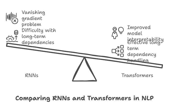
Historically, RNNs, with their inherent design to handle sequential data, were the go-to choice for NLP tasks. Their ability to maintain information across sequences through hidden states provided a sound basis for tasks like text generation and sentiment analysis. However, RNNs, including their advanced variants like LSTM (Long Short-Term Memory) and GRU (Gated Recurrent Units), suffer from significant drawbacks, notably difficulty in capturing long-term dependencies and a propensity for the vanishing gradient problem.
Transformers revolutionized this landscape with the introduction of the attention mechanism, allowing the model to weigh the importance of different words within a sequence regardless of their positional distance. This capability not only addresses the long-term dependency issue but also significantly improves model interpretability.
For instance, when analyzing sentiment, a Transformer can directly correlate adjectives with the subjects they modify, even if several words apart, a task that RNNs find challenging without extensive training and layering.
# Example of Transformer attention mechanism in PyTorch import torch from torch.nn import MultiheadAttention embed_size = 256 num_heads = 8 seq_length = 30 batch_size = 64 # Dummy input: (sequence length, batch size, embedding dimension) src = torch.rand((seq_length, batch_size, embed_size)) # Initialize MultiheadAttention attention = MultiheadAttention(embed_size, num_heads) # Apply attention output, attn_weights = attention(src, src, src)
Efficiency and Training Time
When it comes to training efficiency, Transformers offer a clear advantage due to their parallel processing capability. Unlike RNNs that process data sequentially, Transformers can process entire sequences simultaneously, leveraging modern hardware architectures more effectively. This aspect drastically reduces training time, which is critical for the development lifecycle of NLP models.
However, the efficiency of Transformers comes at a cost of increased computational resource demands due to the attention mechanism’s complexity. Practically, this means developers should be cognizant of memory constraints and possibly leverage strategies such as gradient checkpointing and mixed-precision training to mitigate these issues.
Real-world Application and Scalability
In real-world applications, the choice between RNNs and Transformers often boils down to the scale and nature of the task. For instance, RNNs might still be preferred in scenarios with strict latency requirements or where computing resources are limited, despite their limitations.
Meanwhile, the scalability of Transformers, illustrated by models like GPT (Generative Pretrained Transformer) and BERT (Bidirectional Encoder Representations from Transformers), showcases their superior performance on a wide range of NLP tasks, from language translation to question-answering systems. Their ability to be pre-trained on massive datasets and fine-tuned for specific tasks provides a level of flexibility and efficiency difficult for RNN-based models to match.
As an example, fine-tuning BERT for a sentiment analysis task can be accomplished with relatively few lines of code using libraries like Hugging Face’s Transformers:
from transformers import (
    BertTokenizer,
    BertForSequenceClassification,
    Trainer,
    TrainingArguments
)
import torch


class BertTextClassifier:
    """
    BERT-based text classifier using Hugging Face transformers.
    """

    def __init__(
        self,
        model_name: str = 'bert-base-uncased',
        num_labels: int = 2
    ):
        """
        Initialize the BERT classifier.

        Args:
            model_name (str): Name of the pre-trained BERT model
            num_labels (int): Number of classification labels
        """
        self.tokenizer = BertTokenizer.from_pretrained(model_name)
        self.model = BertForSequenceClassification.from_pretrained(
            model_name,
            num_labels=num_labels
        )

    def prepare_training_args(
        self,
        output_dir: str = './results',
        num_epochs: int = 3,
        batch_size: int = 8,
        warmup_steps: int = 500,
        weight_decay: float = 0.01,
        logging_dir: str = './logs'
    ) -> TrainingArguments:
        """
        Prepare training arguments for the model.

        Args:
            output_dir (str): Directory to save the model
            num_epochs (int): Number of training epochs
            batch_size (int): Batch size for training and evaluation
            warmup_steps (int): Number of warmup steps
            weight_decay (float): Weight decay for optimization
            logging_dir (str): Directory for logging

        Returns:
            TrainingArguments: Configured training arguments
        """
        return TrainingArguments(
            output_dir=output_dir,
            num_train_epochs=num_epochs,
            per_device_train_batch_size=batch_size,
            per_device_eval_batch_size=batch_size,
            warmup_steps=warmup_steps,
            weight_decay=weight_decay,
            logging_dir=logging_dir,
            evaluation_strategy="epoch",  # Changed from evaluate_during_training
            save_strategy="epoch",
            load_best_model_at_end=True,
            metric_for_best_model="loss"
        )

    def tokenize_text(self, text: str) -> dict:
        """
        Tokenize input text for BERT processing.

        Args:
            text (str): Input text to tokenize

        Returns:
            dict: Tokenized input with attention masks
        """
        return self.tokenizer(
            text,
            return_tensors="pt",
            padding=True,
            truncation=True,
            max_length=512
        )

    def setup_trainer(
        self,
        training_args: TrainingArguments,
        train_dataset=None,
        eval_dataset=None
    ) -> Trainer:
        """
        Set up the trainer for model training.

        Args:
            training_args (TrainingArguments): Configured training arguments
            train_dataset: Training dataset
            eval_dataset: Evaluation dataset

        Returns:
            Trainer: Configured trainer object
        """
        return Trainer(
            model=self.model,
            args=training_args,
            train_dataset=train_dataset,
            eval_dataset=eval_dataset
        )


def main():
    """Example usage of BertTextClassifier"""
    # Initialize classifier
    classifier = BertTextClassifier()

    # Example text
    sample_text = "This new AI model is revolutionary."

    # Tokenize input
    inputs = classifier.tokenize_text(sample_text)
    print("Tokenized input:", inputs)

    # Prepare training arguments
    training_args = classifier.prepare_training_args()

    # Setup trainer
    trainer = classifier.setup_trainer(training_args)

    # Note: Actual training would require proper dataset
    print("\nModel and trainer setup complete.")
    print("To train the model, you would need to:")
    print("1. Prepare your dataset")
    print("2. Call trainer.train()")


if __name__ == "__main__":
    main()
Conclusion and Best Practices
In summary, while RNNs have offered foundational advancements in NLP, the advent of Transformers and their superior handling of sequence dependencies, scalability, and efficiency in processing suggest they are better suited for contemporary demands in NLP tasks. For developers, the practical advice would include:
- Leverage the parallel processing and pre-training capabilities of Transformers for large-scale NLP tasks.
- Consider RNNs for scenarios where model simplicity and resource constraints are paramount.
- Stay informed on the evolving landscape of models and optimization techniques to best utilize computational resources.
Ultimately, the choice between Transformers and RNNs should be guided by the specific requirements and constraints of the task at hand, with an emphasis on maximizing performance while managing computational and time resources effectively.
Implementing an RNN Example in Python
Recurrent Neural Networks (RNNs) have been a cornerstone in the field of machine learning for processing sequential data, offering significant advantages in tasks such as language modeling, speech recognition, and time series prediction. In this section, we delve into the practical aspects of implementing a simple RNN model in Python, using TensorFlow and Keras, to give you a hands-on understanding of how RNNs work and how they can be used effectively in your projects.
Understanding RNNs
RNNs are distinct from other neural networks due to their ability to maintain internal state or memory, allowing them to process sequences of inputs. This feature makes RNNs ideal for applications where the temporal sequence of data is critical. However, traditional RNNs are prone to vanishing and exploding gradient problems, impacting their ability to learn long-term dependencies effectively.
Setting Up Your Environment
Before embarking on the coding journey, ensure your Python environment is set up with the necessary libraries. TensorFlow 2.x dramatically simplifies the process of building and training RNN models, thanks to its high-level Keras API. Install TensorFlow by running:
pip install tensorflow
Building a Simple RNN Model in Python
For this example, we’ll construct a model to predict the next number in a sequence. While simplistic, this task encapsulates the essence of RNN functionality.
- Import Necessary Libraries
import tensorflow as tf from tensorflow.keras.models import Sequential from tensorflow.keras.layers import SimpleRNN, Dense
- Prepare the Dataset
Typically, RNNs require data to be in a specific format, usually (samples, time steps, features). For simplicity, let’s generate some sequential data:
import numpy as np

# Generate sequential data: integers from 0 to 99
data = np.arange(100)

# Prepare input (X) and target (y) sequences
X = data[:-1]  # All elements except the last
y = data[1:]   # All elements except the first

# Reshape data to fit model requirements: (samples, time steps, features)
X = X.reshape(len(X), 1, 1)
y = y.reshape(len(y), 1)

# Print shapes for verification
print(f"X shape: {X.shape}")  # (99, 1, 1)
print(f"y shape: {y.shape}") # (99, 1)- Define the RNN Model
We’ll use a simple RNN layer followed by a Dense layer to predict the output. Adjusting the units parameter alters the model’s capacity to learn complex patterns.
from tensorflow.keras.models import Sequential
from tensorflow.keras.layers import SimpleRNN, Dense
from tensorflow.keras.optimizers import Adam


def create_sequence_model(
    input_shape: tuple = (1, 1),
    rnn_units: int = 10,
    output_units: int = 1,
    learning_rate: float = 0.001
) -> Sequential:
    """
    Creates a sequential model with SimpleRNN and Dense layers.

    Args:
        input_shape (tuple): Shape of input data (time_steps, features)
        rnn_units (int): Number of units in the RNN layer
        output_units (int): Number of units in the output layer
        learning_rate (float): Learning rate for Adam optimizer

    Returns:
        Sequential: Compiled Keras sequential model
    """
    # Initialize sequential model
    model = Sequential([
        SimpleRNN(
            units=rnn_units,
            activation='relu',
            input_shape=input_shape,
            name='rnn_layer'
        ),
        Dense(
            units=output_units,
            name='output_layer'
        )
    ])

    # Compile model
    model.compile(
        optimizer=Adam(learning_rate=learning_rate),
        loss='mse',
        metrics=['mae']  # Adding mean absolute error as additional metric
    )

    return model


# Example usage
if __name__ == "__main__":
    # Create model with default parameters
    model = create_sequence_model()

    # Print model summary
    model.summary()

    """
    Example training usage:
    history = model.fit(
        X_train,
        y_train,
        epochs=100,
        batch_size=32,
        validation_split=0.2,
        verbose=1
    )
"""- Train the Model
With data prepared and the model defined, we proceed to train it. The epochs and batch_size parameters can significantly affect training performance and outcomes.
model.fit(X, y, epochs=200, batch_size=16)
- Evaluate and Predict
After training, use the model to make predictions. Here, we predict the next number in the sequence given a new input.
import numpy as np
from typing import Union, List


def predict_next_number(
    model,
    input_number: Union[int, float],
    verbose: bool = True
) -> float:
    """
    Predicts the next number in a sequence using the trained model.

    Args:
        model: Trained keras model
        input_number (Union[int, float]): Input number to predict from
        verbose (bool): Whether to print prediction details

    Returns:
        float: Predicted next number
    """
    # Reshape input for model requirements: (batch_size, time_steps, features)
    test_input = np.array([input_number]).reshape(1, 1, 1)

    # Make prediction
    predicted_number = model.predict(test_input, verbose=0)[0][0]

    if verbose:
        print(f"Input number: {input_number}")
        print(f"Predicted next number: {predicted_number:.2f}")

    return predicted_number


def predict_sequence(
    model,
    start_number: Union[int, float],
    sequence_length: int = 5,
    verbose: bool = True
) -> List[float]:
    """
    Predicts a sequence of numbers starting from a given number.

    Args:
        model: Trained keras model
        start_number (Union[int, float]): Starting number for prediction
        sequence_length (int): Number of predictions to make
        verbose (bool): Whether to print prediction details

    Returns:
        List[float]: List of predicted numbers
    """
    current_number = start_number
    predictions = []

    for i in range(sequence_length):
        predicted = predict_next_number(model, current_number, verbose=False)
        predictions.append(predicted)
        current_number = predicted

    if verbose:
        print(f"Starting number: {start_number}")
        print("Predicted sequence:")
        for i, pred in enumerate(predictions, 1):
            print(f"Step {i}: {pred:.2f}")

    return predictions


# Example usage
if __name__ == "__main__":
    # Assuming we have a trained model
    # Single prediction
    input_number = 100
    prediction = predict_next_number(model, input_number)

    # Sequence prediction
    start_number = 100
    sequence = predict_sequence(
        model,
        start_number,
        sequence_length=5
    )

    # Visualization of predictions
    try:
        import matplotlib.pyplot as plt

        plt.figure(figsize=(10, 6))
        plt.plot(
            range(len(sequence)),
            sequence,
            'b-o',
            label='Predicted Values'
        )
        plt.title('Sequence Prediction')
        plt.xlabel('Step')
        plt.ylabel('Predicted Value')
        plt.grid(True)
        plt.legend()
        plt.show()
    except ImportError:
        print("Matplotlib not installed. Skipping visualization.")
Best Practices and Potential Pitfalls
- Normalization: RNNs are sensitive to the scale of input data. Normalizing data can help improve training efficiency and model accuracy.
- Gradient Clipping: Implementing gradient clipping can mitigate the exploding gradient problem, common in training deep RNNs.
- Sequence Padding: When dealing with variable-length sequences, padding can standardize input shapes. TensorFlow’s pad_sequences utility is particularly useful for this task.
- Choosing the Right Activation: While ReLU activations can accelerate training, they may also lead to the dying ReLU problem. Experiment with activations like tanh or ELU for more stable training.
Conclusion
Through this Python implementation, we’ve explored the basics of constructing and training an RNN model using TensorFlow and Keras. While the example provided is straightforward, it underscores the process and considerations involved in working with RNNs. As you delve into more complex models and datasets, remember the importance of preprocessing, model architecture choices, and the potential need for techniques to combat issues like vanishing or exploding gradients. With these fundamentals, you’re well-equipped to tackle a wide range of sequence modeling problems using RNNs in your machine learning endeavors.
Building a Simple Transformer Model for NLP in Python
In the constantly evolving landscape of machine learning, transformers have emerged as a leading architecture, particularly for natural language processing (NLP) tasks. Unlike Recurrent Neural Networks (RNNs), which process data sequentially, transformers utilize a mechanism known as attention to weigh the importance of different words in a sentence, leading to significant improvements in processing efficiency and performance on complex NLP tasks. This article aims to guide developers through the process of building a simple transformer model in Python, providing the tools necessary to harness the power of this cutting-edge technology.
Understanding the Transformer Architecture
Before diving into code, it’s crucial to understand the basic components of a transformer model. At its core, a transformer consists of an encoder and decoder, each made up of multiple layers that include multi-head self-attention mechanisms and fully connected feed-forward networks. The self-attention mechanism allows the model to weigh the significance of each word in a sentence relative to others, which is key for understanding context and meaning.
Setting the Stage: Prerequisites and Libraries
To begin, ensure you have Python installed along with PyTorch, a popular framework for building deep learning models. PyTorch offers a user-friendly interface for constructing transformers from scratch and also provides pre-built models through its torchtext and transformers libraries.
pip install torch torchvision torchaudio pip install transformers
Implementing a Transformer from Scratch
While leveraging pre-built models can be useful, building a transformer from scratch offers invaluable insights. Below is a simplified example focusing on the conceptual framework rather than optimizing for performance.
- Define the Transformer Block
import torch
import torch.nn as nn
import torch.nn.functional as F


class TransformerBlock(nn.Module):
    def __init__(self, k, heads):
        super().__init__()

        self.att = MultiHeadAttention(heads, k)
        self.ff = nn.Sequential(
            nn.Linear(k, 4 * k),
            nn.ReLU(),
            nn.Linear(4 * k, k)
        )

    def forward(self, x):
        x = self.att(x) + x        # First residual connection
        x = self.ff(x) + x         # Second residual connection
return x- Multi-Head Attention
class MultiHeadAttention(nn.Module):
    def __init__(self, heads, k):
        super().__init__()

        # Save dimensions
        self.k = k
        self.heads = heads

        # Linear transformations for keys, queries, and values
        self.tokeys = nn.Linear(k, k * heads, bias=False)
        self.toqueries = nn.Linear(k, k * heads, bias=False)
        self.tovalues = nn.Linear(k, k * heads, bias=False)

        # Final linear transformation to combine heads
        self.unifyheads = nn.Linear(heads * k, k)

    def forward(self, x):
        # Input dimensions
        b, t, k = x.size()  # batch_size, sequence_length, embedding_dim
        h = self.heads

        # Transform input into keys, queries and values
        keys = self.tokeys(x).view(b, t, h, k)
        queries = self.toqueries(x).view(b, t, h, k)
        values = self.tovalues(x).view(b, t, h, k)

        # Scaled dot-product attention...
        # [Your implementation here]

return output- Positional Encoding
class PositionalEncoder(nn.Module):
    def __init__(self, d_model, max_seq_len=80):
        super().__init__()

        self.d_model = d_model

        # Create constant positional encoding matrix
        pe = torch.zeros(max_seq_len, d_model)

        # Calculate positional encodings
        for pos in range(max_seq_len):
            for i in range(0, d_model, 2):
                # Sine for even indices
                pe[pos, i] = math.sin(
                    pos / (10000 ** ((2 * i) / d_model))
                )
                # Cosine for odd indices
                pe[pos, i + 1] = math.cos(
                    pos / (10000 ** ((2 * i + 1) / d_model))
                )

        # Add batch dimension
        pe = pe.unsqueeze(0)

        # Register buffer (persistent state)
        self.register_buffer('pe', pe)

    def forward(self, x):
        # Add positional encoding to input
        x = x + Variable(
            self.pe[:, :x.size(1)],
            requires_grad=False
        )
return x- Assembling the Transformer Model
class Transformer(nn.Module):
    def __init__(
        self,
        d_model=512,
        n_heads=8,
        n_layers=6,
        max_seq_len=80,
        dropout=0.1
    ):
        super().__init__()

        # Positional encoding layer
        self.positional_encoder = PositionalEncoder(
            d_model=d_model,
            max_seq_len=max_seq_len
        )

        # Stack of transformer blocks
        self.transformer_blocks = nn.ModuleList([
            TransformerBlock(
                k=d_model,
                heads=n_heads
            ) for _ in range(n_layers)
        ])

        # Dropout for regularization
        self.dropout = nn.Dropout(dropout)

    def forward(self, x):
        # Add positional encoding
        x = self.positional_encoder(x)

        # Apply dropout
        x = self.dropout(x)

        # Pass through transformer blocks
        for block in self.transformer_blocks:
            x = block(x)

        return x
Best Practices and Potential Pitfalls
Constructing a transformer model in Python, particularly from scratch, can yield profound insights but also comes with its challenges. It is critical to pay attention to the model’s dimensionality at each layer, ensuring consistency throughout. Debugging dimensionality issues early can save considerable time. Additionally, initializing model weights properly is critical for achieving convergence during training.
Training transformers requires substantial computational resources, especially as the complexity of the task increases. Utilizing specialized hardware, such as GPUs, and leveraging parallel processing frameworks can vastly improve training efficiency.
Conclusion
Building a transformer model in Python is a rewarding venture that can substantially improve the performance of NLP tasks. While this guide provided a foundational starting point, the scalability and versatility of transformers allow for extensive customization and optimization tailored to specific problems. Embracing the transformer architecture signifies a step towards the forefront of artificial intelligence innovations, opening a plethora of opportunities in machine learning and beyond.
Best Practices for Developing with RNNs and Transformers
In the dynamic world of machine learning, Recurrent Neural Networks (RNNs) and Transformers have emerged as powerful models for handling sequential data. Each with their unique strengths and challenges, determining the best practices for development with these architectures is essential for maximizing performance and efficiency. This section delves into the key considerations, practical advice, and examples in Python to guide developers through the intricate process of working with RNNs and Transformers.
RNNs: Mastering Sequential Data Processing
RNNs are famed for their ability in processing sequences, such as text or time series data, by maintaining a memory of previous inputs. However, they are also notorious for difficulties in training, primarily due to issues like vanishing and exploding gradients.
- Gradient Clipping: Implement gradient clipping to combat exploding gradients. This technique limits the size of gradients to a small range to prevent drastic updates to model parameters. In PyTorch, you can apply gradient clipping using torch.nn.utils.clip_grad_norm_ as follows:torch.nn.utils.clip_grad_norm_(model.parameters(), max_norm=1.0)
- Choice of Activation Function: Use ReLU or its variants like LeakyReLU to mitigate vanishing gradients. Unlike sigmoid or tanh, ReLU provides a non-saturating nonlinearity, which helps in maintaining the gradient flow.
- Gated Units for Memory Management: Prefer gated units such as LSTM or GRU over vanilla RNNs. These units introduce gates that effectively regulate the flow of information, making them more apt at capturing long-term dependencies and alleviating vanishing gradient issues. The following code snippet demonstrates initializing an LSTM layer in PyTorch:lstm_layer = nn.LSTM(input_size=100, hidden_size=50, num_layers=2, batch_first=True)
Transformers: Elevating the Standards of Parallel Processing
Transformers revolutionized the field by introducing self-attention mechanisms, enabling models to weigh the importance of different parts of the input data differently. This architecture excels in tasks requiring understanding of the entire context, such as language understanding and generative tasks.
- Attention Is All You Need: Leverage the power of the attention mechanism which allows models to focus on relevant parts of the input data. The implementation of a self-attention layer in TensorFlow is straightforward with the MultiHeadAttention class:from tensorflow.keras.layers import MultiHeadAttention mha = MultiHeadAttention(key_dim=2, num_heads=2)
- Positional Encoding Is Crucial: Since Transformers do not inherently process data in sequence, positional encoding is necessary to provide the model with the information about the order of the sequence. This can be implemented by adding a positional encoding vector to the input embeddings.
- Efficient Batching and Padding: When training Transformers, organize your data into batches efficiently. Pad sequences to uniform length in each batch, and consider using dynamic padding to minimize the number of padded tokens. This is crucial for optimizing computational resources.
- Regularization and Dropout: To prevent overfitting, especially given the Transformer’s capacity for large-scale parameterization, apply dropout in the attention layers and between sub-layers in the encoder and decoder stacks. For instance, within TensorFlow:transformer_layer = layers.Transformer(num_heads=2, key_dim=2, dropout=0.1)
Common Ground: Optimizations and Implementation Tips
For both architectures, certain practices are universally beneficial:
- Use Pre-trained Models When Possible: Leverage pre-trained models available in libraries such as Hugging Face’s Transformers. Fine-tuning a pre-trained model on your specific dataset can drastically reduce training time and resource consumption, while achieving high performance.
- Optimize Data Processing: Utilize efficient data loading and preprocessing techniques. Tools like TensorFlow’s tf.data API or PyTorch’s DataLoader class can significantly improve IO bottlenecks.
- Experiment with Learning Rate Schedulers: Implement learning rate schedulers such as the cyclic learning rate or learning rate warmup. They can help in achieving faster convergence and improve model performance.scheduler = torch.optim.lr_scheduler.CyclicLR(optimizer, base_lr=0.001, max_lr=0.01)
- Monitor and Debug: Utilize tools like TensorBoard or Weights & Biases for monitoring training progress, debugging issues, and comparing experiments. Visualizing model internals and metrics can provide insights into model behavior and performance bottlenecks.
In conclusion, effective development with RNNs and Transformers necessitates a deep understanding of both models’ intricacies and a strategic approach to model design, training, and optimization. By adhering to these best practices and utilizing the provided Python code examples as starting points, developers can enhance their machine learning projects, leading to more robust, efficient, and high-performing models.
Overcoming Common Challenges in RNN and Transformer Implementations
The advent of Recurrent Neural Networks (RNNs) and Transformers has revolutionized how machine learning models process sequential data, such as texts and time series. However, implementing these architectures effectively involves overcoming specific challenges. This section delves into the intricacies of RNN and Transformer models, highlighting common pitfalls and offering practical solutions tailored for developers.
Vanishing and Exploding Gradients in RNNs
A notorious issue with standard RNNs is the vanishing and exploding gradient problem, which hampers the network’s ability to learn long-range dependencies. These phenomena occur due to the repetitive nature of gradient computation through time, leading to gradients that either diminish or grow exponentially.
Solution: To counteract these issues, Long Short-Term Memory (LSTM) units or Gated Recurrent Units (GRUs) are often utilized. They introduce gates that regulate the flow of information, making it easier for the network to capture long-term dependencies without losing crucial information over time. Here’s an illustrative Python snippet using LSTM:
from keras.models import Sequential from keras.layers import LSTM, Dense model = Sequential([ LSTM(100, return_sequences=True, input_shape=(timesteps, features)), LSTM(100), Dense(output_size), ])
This example demonstrates a basic LSTM-based model capable of mitigating the vanishing gradient problem, thereby stabilizing training.
Handling Large Sequences in Transformers
Transformers, unlike RNNs, can process entire sequences simultaneously, which enables unparalleled parallelization and efficiency. However, this comes at a cost: the self-attention mechanism scales quadratically with the sequence length, posing a considerable challenge for long sequences.
Solution: Efficient attention mechanisms, such as the Longformer or Linformer, propose ways to reduce the computational complexity from quadratic to linear with respect to sequence length. Implementing these mechanisms can significantly reduce memory consumption and computational time. For example, using the Longformer from the Hugging Face Transformers library:
from transformers import LongformerModel, LongformerTokenizer tokenizer = LongformerTokenizer.from_pretrained(’allenai/longformer-base-4096′) model = LongformerModel.from_pretrained(’allenai/longformer-base-4096′) input_ids = tokenizer.encode(„Your long sequence here”, return_tensors=”pt”) output = model(input_ids)
In this code, LongformerModel is adept at processing much longer sequences than the standard Transformer model, making it ideal for tasks like document classification or summarization where context length is crucial.
Optimizing Memory and Computational Efficiency
Both RNNs and Transformers are resource-intensive, requiring substantial memory and computational power, especially for large models or datasets.
For RNNs, a practical tip is to use batch processing and truncated backpropagation through time (TBPTT). TBPTT involves splitting the input sequences into smaller segments, which reduces the computation load while still allowing effective learning across sequence chunks.
For Transformers, leveraging mixed-precision training can lead to significant performance improvements. This approach utilizes both 16-bit and 32-bit floating-point arithmetic during different phases of training, balancing precision and computational efficiency.
Example of enabling mixed-precision training with TensorFlow:
from tensorflow.keras.mixed_precision import experimental as mixed_precision policy = mixed_precision.Policy(’mixed_float16′) mixed_precision.set_policy(policy)
This code snippet configures TensorFlow to use mixed precision, which can accelerate training times on compatible hardware without a significant loss in model accuracy.
Regularization and Overfitting
Especially with complex models like Transformers, overfitting — where a model learns the training data too well and fails to generalize to unseen data — can be a concern.
Solution: Employing techniques such as dropout, weight decay (L2 regularization), and attention dropout in Transformers are effective methods to combat overfitting. Here’s an example of incorporating dropout in a Transformer model layer:
from keras.layers import Dropout, LayerNormalization def transformer_encoder_layer(inputs): # Your Transformer implementation here outputs = Dropout(0.1)(inputs) outputs = LayerNormalization()(outputs + inputs) return outputs
In this function, Dropout is applied to the inputs of a Transformer encoder layer, introducing regularization by randomly setting a portion of the input units to 0 at each update during training.
Conclusion
Overcoming implementation challenges in RNN and Transformer models is essential for harnessing their full potential in sequential data tasks. Through architectural modifications like LSTMs and GRUs for RNNs, adopting efficient attention mechanisms for Transformers, and employing smart training strategies such as mixed-precision training and dropout for regularization, developers can build more robust, efficient, and effective models. The key is a thorough understanding of each model’s intricacies and a thoughtful application of best practices tailored to your specific use case.
The Future of AI: Predictions on the Evolving Role of RNNs and Transformers
The landscape of artificial intelligence (AI) is continually evolving, with models and algorithms becoming more sophisticated each year. Two of the most influential architectures in this development have been Recurrent Neural Networks (RNNs) and Transformers. Both have played pivotal roles in advancing natural language processing (NLP) and other areas of machine learning. However, as we look to the future, the trajectory for these technologies seems to diverge, with Transformers poised to dominate. This prediction is not without its nuances, and understanding the evolving role of RNNs and Transformers requires a deep dive into their capabilities, limitations, and potential future applications.
RNNs: Challenges and Niche Adoption
RNNs were a cornerstone in early NLP advancements due to their sequential data processing capability, effectively handling tasks such as language modeling and translation. Despite their initial success, RNNs face significant challenges:
- Vanishing Gradient Problem: During backpropagation, RNNs can suffer from vanishing gradients, making it hard to learn long-term dependencies in data.
- Sequential Computation: The inherent sequential nature of RNNs limits parallelization, which becomes a bottleneck in training on large datasets.
Nevertheless, RNNs aren’t obsolete. They remain effective in niche applications where complex, time-series data requires detailed analysis. For developers, leveraging RNNs in such contexts means carefully managing gradient flow, possibly incorporating techniques like gating (as in LSTM and GRU models) to mitigate vanishing gradients. Consider the following LSTM example for time-series prediction:
from keras.models import Sequential from keras.layers import LSTM, Dense model = Sequential() model.add(LSTM(50, activation=’relu’, input_shape=(time_steps, n_features))) model.add(Dense(1)) model.compile(optimizer=’adam’, loss=’mse’)
This code constructs a simple LSTM model for time-series data, highlighting RNNs’ continued relevance in specific domains.
Transformers: Setting the Standard
Transformers have fundamentally altered the AI landscape since their introduction. Their key innovations—self-attention and parallel processing capabilities—address many of RNNs’ limitations, enabling models to learn dependencies regardless of sequence length without being hampered by the sequential computation.
The success of models like BERT, GPT (in various iterations), and T5 across a multitude of NLP benchmarks have set transformers as the standard approach for most modern NLP tasks. Their architecture not only facilitates a more profound understanding of language nuances but also enables a broader application in generating human-like text, answering questions, and more.
Practical Advice for Developers
When building solutions with transformers, developers should:
- Leverage Pre-trained Models: Utilizing models like GPT-3 or BERT as a base can significantly reduce development time and computing resources.
- Fine-tuning: Adjusting the final layers of a pre-trained transformer to suit specific tasks can optimize performance without the need for training the model from scratch.
Consider the following example of fine-tuning BERT for a sentiment analysis task using Hugging Face’s transformers library:
from transformers import BertTokenizer, TFBertForSequenceClassification from transformers import InputExample, InputFeatures model = TFBertForSequenceClassification.from_pretrained(„bert-base-uncased”) tokenizer = BertTokenizer.from_pretrained(„bert-base-uncased”) # Define your process_data function and other preprocessing tasks here train_dataset = process_data(train_examples, tokenizer) model.fit(train_dataset, epochs=2, batch_size=8)
This snippet illustrates how one might fine-tune BERT for a specific application with minimal code, by utilizing pre-trained components and focusing on the data and task-specific tuning.
Looking Ahead
The trajectory of NLP and AI as a whole is unmistakably leaning towards transformer models, primarily due to their scalability, efficiency, and superior handling of context in language tasks. That said, the nuanced capabilities of RNNs in processing sequential, time-series data ensure they remain valuable in specific scenarios.
For developers in the AI space, staying informed about the latest research and developments is crucial. The interplay between evolving technologies like RNNs and transformers offers a rich set of tools for tackling complex problems. As we push the boundaries of what AI can achieve, understanding the strengths and limitations of these architectures will be paramount in crafting innovative solutions that can understand, interpret, and generate human language with unprecedented acuity.
FAQ
What are RNNs and why are they important in AI?
Recurrent Neural Networks (RNNs) are a class of artificial neural networks where connections between nodes form a directed graph along a temporal sequence. This design allows RNNs to exhibit temporal dynamic behavior and process sequences of inputs, making them essential for tasks such as language modeling, speech recognition, and time series prediction.
How do Transformers differ from RNNs in Machine Learning?
Transformers abandon the sequential processing of RNNs for a parallel approach, utilizing self-attention mechanisms to weigh the significance of different parts of the input data differently. This allows Transformers to process all parts of the sequence simultaneously, leading to significant improvements in processing speed and effectiveness, particularly in tasks related to natural language processing (NLP) and computer vision.
Why have Transformers become more popular than RNNs for certain AI tasks?
Transformers have gained popularity over RNNs for tasks like text translation, content generation, and even in non-language tasks, because they can handle long sequences of data more efficiently and with greater accuracy. Their ability to process input data in parallel rather than sequentially allows for faster training times and better performance on tasks requiring an understanding of context within large datasets.
Can Transformers be used for tasks other than NLP?
Yes, while Transformers were initially designed for natural language processing tasks, their architecture allows them to be adapted for a variety of other applications. This includes fields like computer vision, where they can be used for image recognition and generation, and even in areas such as protein structure prediction, demonstrating their versatility and effectiveness outside of NLP.
What are the main challenges associated with RNNs that Transformers aim to solve?
The main challenges associated with RNNs include difficulty in training over long sequences due to issues like vanishing gradients and a fundamentally sequential computation model that doesn’t parallelize well. Transformers address these challenges with their attention mechanisms that capture dependencies without regard to their distance in the input sequence and their inherently parallel structure, leading to more efficient computation and improved performance on tasks requiring long context.
How do Transformers achieve understanding of sequence context?
Transformers employ a mechanism known as self-attention, which allows each element in the input sequence to be associated with every other element, weighted by their relevance. This enables the model to understand the context of each element within the whole sequence effectively, regardless of positional distance, leading to a more nuanced understanding of the sequence as a whole.
What advancements in AI might we see as a result of the continued development of Transformer models?
As Transformer models continue to evolve, we can expect advancements in AI including more sophisticated natural language understanding and generation, more accurate and efficient machine translation, progress in non-language tasks like image and video processing, and new applications in fields like healthcare, autonomous vehicles, and augmented reality. Their flexibility and efficiency make them a driving force for innovation in AI.
AI Agents: Distributed Systems