
Introduction to Generative Models
Generative models are a cornerstone of modern artificial intelligence, enabling machines to create new data that resembles existing datasets. Unlike traditional discriminative models, which focus on classifying or predicting outcomes based on input data, generative models learn the underlying distribution of the data itself. This allows them to generate new, synthetic examples that are statistically similar to the original data. In this section, we will explore what generative models are, compare two of the most popular types—GANs and VAEs—and discuss their applications in today’s AI landscape.
1.1 What Are Generative Models?
A generative model is a type of machine learning model that can generate new data points by learning the probability distribution of a given dataset. In simple terms, after being trained on a dataset (such as images, text, or audio), a generative model can produce new samples that look like they could have come from the original dataset.
For example, if a generative model is trained on thousands of images of handwritten digits, it can create entirely new images of digits that are not present in the training set but still look realistic.
Generative models are fundamentally different from discriminative models, which learn the boundary between classes (e.g., is this image a cat or a dog?). Instead, generative models focus on understanding how the data is structured and how new data can be synthesized.
1.2 Overview: GANs vs. VAEs
Two of the most influential generative models in recent years are Generative Adversarial Networks (GANs) and Variational Autoencoders (VAEs). Both have unique architectures and learning strategies, but they share the common goal of generating new, high-quality data.
GANs (Generative Adversarial Networks):
GANs consist of two neural networks—the generator and the discriminator—that compete in a zero-sum game. The generator tries to create data that is indistinguishable from real data, while the discriminator attempts to distinguish between real and generated data. Through this adversarial process, the generator learns to produce increasingly realistic samples.
VAEs (Variational Autoencoders):
VAEs are based on the autoencoder architecture but introduce a probabilistic approach to encoding and decoding data. Instead of mapping inputs to fixed points in a latent space, VAEs map them to distributions, allowing for smooth sampling and interpolation. VAEs optimize a loss function that balances reconstruction accuracy and the regularization of the latent space, making them powerful for generating new data and exploring the structure of the data manifold.
Key Differences:
While both models are used for data generation, GANs are known for producing sharper and more realistic images, but can be harder to train due to instability. VAEs, on the other hand, offer more stable training and better control over the latent space, but sometimes generate blurrier outputs.
1.3 Applications in Modern AI
Generative models have revolutionized many areas of artificial intelligence and have a wide range of practical applications, including:
Image Synthesis: Creating realistic images, faces, or objects that never existed before. GANs are widely used for generating high-resolution images and deepfakes.
Data Augmentation: Generating additional training data to improve the performance of machine learning models, especially when real data is scarce.
Anomaly Detection: Modeling the normal data distribution allows generative models to identify outliers or anomalies in datasets, which is useful in fraud detection and industrial monitoring.
Text and Audio Generation: Producing human-like text, music, or speech. VAEs and GANs are used in natural language processing and audio synthesis.
Drug Discovery and Design: Generating new molecular structures with desired properties, accelerating the process of finding new drugs.
Understanding GANs (Generative Adversarial Networks)
Generative Adversarial Networks (GANs) have become one of the most influential innovations in the field of artificial intelligence. Introduced by Ian Goodfellow and his colleagues in 2014, GANs have set new standards for generating realistic synthetic data, especially images. In this section, we will explore the architecture and core concepts of GANs, explain how the generator and discriminator interact, and highlight common use cases where GANs excel.
2.1 Architecture and Core Concepts
At the heart of a GAN are two neural networks: the generator and the discriminator. These networks are trained simultaneously in a process that can be likened to a game between two players with opposing goals.
Generator (G): The generator’s job is to create synthetic data that resembles the real data as closely as possible. It takes random noise as input and transforms it into data samples (for example, images).
Discriminator (D): The discriminator’s task is to distinguish between real data (from the training set) and fake data (produced by the generator). It outputs a probability indicating whether a given sample is real or generated.
2.2 How GANs Work: Generator and Discriminator
The training of GANs involves alternating updates to the generator and discriminator:
Step 1: The generator creates a batch of fake data from random noise.
Step 2: The discriminator evaluates both real data and the fake data, outputting probabilities for each.
Step 3: The discriminator is updated to better distinguish real from fake data.
Step 4: The generator is updated to produce more realistic data, aiming to „fool” the discriminator.
This process repeats for many iterations. Over time, the generator becomes better at producing realistic data, while the discriminator becomes more skilled at detecting fakes. Ideally, the generator’s outputs become so convincing that the discriminator cannot reliably tell the difference between real and generated data.
Python Example: Simple GAN Structure
Below is a simplified example of how you might define the generator and discriminator using TensorFlow and Keras:
python

import tensorflow as tf

from tensorflow.keras import layers

# Generator model

def build_generator(latent_dim):

    model = tf.keras.Sequential([

        layers.Dense(128, activation='relu', input_dim=latent_dim),

        layers.Dense(784, activation='sigmoid')  # For MNIST (28x28 images)

    ])

    return model

# Discriminator model

def build_discriminator():

    model = tf.keras.Sequential([

        layers.Dense(128, activation='relu', input_dim=784),

        layers.Dense(1, activation='sigmoid')

    ])

    return model

latent_dim = 100

generator = build_generator(latent_dim)

discriminator = build_discriminator()
This code sets up the basic structure for a GAN that could be trained on the MNIST dataset of handwritten digits.
2.3 Common Use Cases
GANs have found applications in a wide range of fields, thanks to their ability to generate high-quality synthetic data. Some of the most notable use cases include:
Image Generation: GANs can create realistic images of faces, objects, and scenes that never existed. Projects like StyleGAN have demonstrated the ability to generate photorealistic human faces.
Image-to-Image Translation: GANs can transform images from one domain to another, such as turning sketches into photos, black-and-white images into color, or day scenes into night. The Pix2Pix and CycleGAN frameworks are popular for these tasks.
Data Augmentation: In scenarios where real data is limited, GANs can generate additional training samples to improve the performance of machine learning models.
Super-Resolution: GANs can enhance the resolution of images, making them sharper and more detailed.
Art and Creativity: Artists and designers use GANs to create new artworks, music, and even fashion designs by exploring the latent space of generative models.
GANs continue to push the boundaries of what is possible in AI-generated content, making them a vital tool for advanced programmers and researchers.
Understanding VAEs (Variational Autoencoders)
Variational Autoencoders (VAEs) are a powerful class of generative models that combine principles from deep learning and probabilistic graphical models. They are widely used for generating new data, learning meaningful latent representations, and exploring the structure of complex datasets. In this section, we will discuss the architecture and core concepts of VAEs, explain the role of the latent space, and highlight common use cases.
3.1 Architecture and Core Concepts
A Variational Autoencoder consists of two main components: the encoder and the decoder. The architecture is inspired by traditional autoencoders but introduces a probabilistic approach to encoding and decoding data.
Encoder: The encoder network takes input data and maps it to a probability distribution in a lower-dimensional latent space. Instead of producing a single point, the encoder outputs parameters (mean and variance) of a Gaussian distribution for each input.
Latent Space: The latent space is a compressed, abstract representation of the input data. Each point in this space corresponds to a possible data sample.
Decoder: The decoder network samples a point from the latent space and reconstructs the original data from this point.
The key innovation in VAEs is the use of variational inference. During training, the model learns to approximate the true data distribution by optimizing a loss function that combines two terms: the reconstruction loss (how well the output matches the input) and the Kullback-Leibler (KL) divergence (how close the learned latent distribution is to a standard normal distribution).
3.2 The Role of Latent Space
The latent space in a VAE is a continuous, multidimensional space where each point represents a possible data sample. This space is structured so that similar points correspond to similar data, enabling smooth interpolation and exploration.
Key properties of the latent space:
Continuity: Small changes in the latent variables result in small changes in the generated data. This allows for smooth transitions between samples.
Regularization: The KL divergence term in the loss function encourages the latent space to follow a standard normal distribution, preventing overfitting and ensuring that the space is well-organized.
Sampling: New data can be generated by sampling random points from the latent space and passing them through the decoder.
This structure makes VAEs particularly useful for tasks that require understanding or manipulating the underlying factors of variation in the data.
3.3 Common Use Cases
VAEs have a wide range of applications in machine learning and artificial intelligence, including:
Data Generation: VAEs can generate new, realistic samples similar to the training data, such as images, audio, or text.
Dimensionality Reduction: The encoder compresses high-dimensional data into a lower-dimensional latent space, which can be used for visualization or as input to other models.
Anomaly Detection: By modeling the normal data distribution, VAEs can identify outliers or anomalies that do not fit the learned patterns.
Representation Learning: The latent space learned by a VAE often captures meaningful features of the data, which can be useful for downstream tasks like clustering or classification.
Image Editing and Interpolation: Because the latent space is continuous and structured, it is possible to interpolate between different data points, enabling smooth morphing or editing of images.
Python Example: Simple VAE Structure
Below is a basic example of how to define the encoder and decoder for a VAE using TensorFlow and Keras:
python

import tensorflow as tf

from tensorflow.keras import layers

latent_dim = 2  # Size of the latent space

# Encoder

encoder_inputs = tf.keras.Input(shape=(784,))

x = layers.Dense(256, activation='relu')(encoder_inputs)

z_mean = layers.Dense(latent_dim, name='z_mean')(x)

z_log_var = layers.Dense(latent_dim, name='z_log_var')(x)

# Sampling function

def sampling(args):

    z_mean, z_log_var = args

    epsilon = tf.random.normal(shape=(tf.shape(z_mean)[0], latent_dim))

    return z_mean + tf.exp(0.5 * z_log_var) * epsilon

z = layers.Lambda(sampling, output_shape=(latent_dim,), name='z')([z_mean, z_log_var])

encoder = tf.keras.Model(encoder_inputs, [z_mean, z_log_var, z], name='encoder')

# Decoder

latent_inputs = tf.keras.Input(shape=(latent_dim,))

x = layers.Dense(256, activation='relu')(latent_inputs)

decoder_outputs = layers.Dense(784, activation='sigmoid')(x)

decoder = tf.keras.Model(latent_inputs, decoder_outputs, name='decoder')
This code provides the foundation for building and training a VAE on datasets like MNIST.
Implementing GANs in Python
Implementing Generative Adversarial Networks (GANs) in Python is a practical way to understand their inner workings and experiment with generative modeling. In this section, you’ll learn how to set up your environment, build a simple GAN step by step, and train and evaluate your model using Python and popular deep learning libraries.
4.1 Setting Up the Environment
To implement GANs efficiently, you’ll need a Python environment with the following libraries:
TensorFlow or PyTorch (for building and training neural networks)
NumPy (for numerical operations)
Matplotlib (for visualizing results)
scikit-learn (optional, for data preprocessing)
You can install the required packages using pip:
bash

pip install tensorflow numpy matplotlib
For PyTorch users, replace tensorflow with torch and torchvision.
4.2 Step-by-Step GAN Implementation (with Code)
Let’s walk through a minimal GAN implementation using TensorFlow and Keras, focusing on generating handwritten digits from the MNIST dataset.
1. Import Libraries and Load Data
python

import numpy as np

import tensorflow as tf

from tensorflow.keras import layers

import matplotlib.pyplot as plt

# Load and preprocess MNIST data

(x_train, _), (_, _) = tf.keras.datasets.mnist.load_data()

x_train = x_train.astype('float32') / 255.0

x_train = x_train.reshape(-1, 28*28)
2. Build the Generator
python

def build_generator(latent_dim):

    model = tf.keras.Sequential([

        layers.Dense(128, activation='relu', input_dim=latent_dim),

        layers.Dense(784, activation='sigmoid')

    ])

    return model

latent_dim = 100

generator = build_generator(latent_dim)
3. Build the Discriminator
python

def build_discriminator():

    model = tf.keras.Sequential([

        layers.Dense(128, activation='relu', input_dim=784),

        layers.Dense(1, activation='sigmoid')

    ])

    return model

discriminator = build_discriminator()

discriminator.compile(optimizer='adam', loss='binary_crossentropy', metrics=['accuracy'])
4. Combine Models to Form the GAN
python

# Freeze discriminator weights during generator training

discriminator.trainable = False

gan_input = tf.keras.Input(shape=(latent_dim,))

generated_image = generator(gan_input)

gan_output = discriminator(generated_image)

gan = tf.keras.Model(gan_input, gan_output)

gan.compile(optimizer='adam', loss='binary_crossentropy')
5. Training Loop
python

batch_size = 64

epochs = 10000

for epoch in range(epochs):

    # Train discriminator

    idx = np.random.randint(0, x_train.shape[0], batch_size)

    real_imgs = x_train[idx]

    noise = np.random.normal(0, 1, (batch_size, latent_dim))

    fake_imgs = generator.predict(noise)

    d_loss_real = discriminator.train_on_batch(real_imgs, np.ones((batch_size, 1)))

    d_loss_fake = discriminator.train_on_batch(fake_imgs, np.zeros((batch_size, 1)))

    # Train generator

    noise = np.random.normal(0, 1, (batch_size, latent_dim))

    g_loss = gan.train_on_batch(noise, np.ones((batch_size, 1)))

    if epoch % 1000 == 0:

        print(f"Epoch {epoch}, D Loss: {0.5 * np.add(d_loss_real, d_loss_fake)}, G Loss: {g_loss}")
6. Visualize Generated Images
python

def plot_generated_images(generator, latent_dim, n=10):

    noise = np.random.normal(0, 1, (n, latent_dim))

    gen_imgs = generator.predict(noise)

    gen_imgs = gen_imgs.reshape(n, 28, 28)

    plt.figure(figsize=(10, 1))

    for i in range(n):

        plt.subplot(1, n, i+1)

        plt.imshow(gen_imgs[i], cmap='gray')

        plt.axis('off')

    plt.show()

plot_generated_images(generator, latent_dim)
4.3 Training and Evaluating a GAN
Training GANs is a delicate process that requires balancing the learning of both the generator and the discriminator. Some practical tips include:
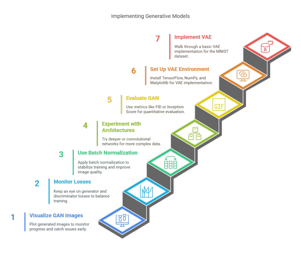
Monitor Losses: Keep an eye on both generator and discriminator losses. If one model becomes too strong, training can stall.
Use Batch Normalization: This can help stabilize training and improve the quality of generated images.
Experiment with Architectures: Try deeper or convolutional networks for more complex data.
Visualize Outputs Regularly: Plot generated samples during training to monitor progress and catch issues early.
Evaluation:
Unlike traditional models, GANs are not evaluated with accuracy or loss alone. Visual inspection of generated samples is common, but you can also use metrics like the Fréchet Inception Distance (FID) or Inception Score for quantitative evaluation.
Implementing VAEs in Python
Variational Autoencoders (VAEs) are a popular choice for generative modeling, offering a principled approach to learning latent representations and generating new data. In this section, you’ll learn how to set up your environment, implement a simple VAE step by step, and train and evaluate your model using Python and TensorFlow/Keras.
5.1 Setting Up the Environment
To implement a VAE, you’ll need a Python environment with the following libraries:
TensorFlow (for building and training neural networks)
NumPy (for numerical operations)
Matplotlib (for visualizing results)
Install the required packages using pip:
bash

pip install tensorflow numpy matplotlib

5.2 Step-by-Step VAE Implementation
Let’s walk through a basic VAE implementation for the MNIST dataset.
1. Import Libraries and Load Data
python

import numpy as np

import tensorflow as tf

from tensorflow.keras import layers

import matplotlib.pyplot as plt

# Load and preprocess MNIST data

(x_train, _), (_, _) = tf.keras.datasets.mnist.load_data()

x_train = x_train.astype('float32') / 255.0

x_train = x_train.reshape(-1, 28*28)
2. Build the Encoder
python

latent_dim = 2  # Size of the latent space

encoder_inputs = tf.keras.Input(shape=(784,))

x = layers.Dense(256, activation='relu')(encoder_inputs)

z_mean = layers.Dense(latent_dim, name='z_mean')(x)

z_log_var = layers.Dense(latent_dim, name='z_log_var')(x)

def sampling(args):

    z_mean, z_log_var = args

    epsilon = tf.random.normal(shape=(tf.shape(z_mean)[0], latent_dim))

    return z_mean + tf.exp(0.5 * z_log_var) * epsilon

z = layers.Lambda(sampling, output_shape=(latent_dim,), name='z')([z_mean, z_log_var])

encoder = tf.keras.Model(encoder_inputs, [z_mean, z_log_var, z], name='encoder')
3. Build the Decoder
python

latent_inputs = tf.keras.Input(shape=(latent_dim,))

x = layers.Dense(256, activation='relu')(latent_inputs)

decoder_outputs = layers.Dense(784, activation='sigmoid')(x)

decoder = tf.keras.Model(latent_inputs, decoder_outputs, name='decoder')
4. Build the VAE Model
python

outputs = decoder(encoder(encoder_inputs)[2])

vae = tf.keras.Model(encoder_inputs, outputs, name='vae')
5. Define the VAE Loss
python

reconstruction_loss = tf.keras.losses.binary_crossentropy(encoder_inputs, outputs)

reconstruction_loss = tf.reduce_sum(reconstruction_loss, axis=1)

kl_loss = -0.5 * tf.reduce_sum(1 + z_log_var - tf.square(z_mean) - tf.exp(z_log_var), axis=1)

vae_loss = tf.reduce_mean(reconstruction_loss + kl_loss)

vae.add_loss(vae_loss)

vae.compile(optimizer='adam')
6. Train the VAE
python

vae.fit(x_train, x_train, epochs=30, batch_size=128)
5.3 Training and Evaluating a VAE
Training a VAE involves optimizing both the reconstruction loss and the KL divergence to ensure the model learns a meaningful latent space and can generate realistic data.
Evaluation Tips:
Visualize Reconstructions: Compare original and reconstructed images to assess how well the VAE captures data features.
Sample from Latent Space: Generate new images by sampling random points from the latent space and passing them through the decoder.
Latent Space Exploration: For low-dimensional latent spaces (e.g., 2D), visualize how different regions correspond to different types of generated data.
Example: Visualizing Generated Digits
python

def plot_latent_space(decoder, n=15, digit_size=28):

    # Display a n*n 2D manifold of digits

    grid_x = np.linspace(-3, 3, n)

    grid_y = np.linspace(-3, 3, n)[::-1]

    figure = np.zeros((digit_size * n, digit_size * n))

    for i, yi in enumerate(grid_y):

        for j, xi in enumerate(grid_x):

            z_sample = np.array([[xi, yi]])

            x_decoded = decoder.predict(z_sample)

            digit = x_decoded[0].reshape(digit_size, digit_size)

            figure[i * digit_size: (i + 1) * digit_size,

                   j * digit_size: (j + 1) * digit_size] = digit

    plt.figure(figsize=(10, 10))

    plt.imshow(figure, cmap='Greys_r')

    plt.axis('off')

    plt.show()

plot_latent_space(decoder)
Comparing GANs and VAEs: Strengths and Weaknesses
Generative Adversarial Networks (GANs) and Variational Autoencoders (VAEs) are two of the most popular generative models in deep learning. While both are designed to generate new data similar to a training set, they differ significantly in their architectures, training processes, and the quality of their outputs. In this section, we will compare GANs and VAEs in terms of the quality of generated data, training stability, and practical considerations for advanced programmers.
6.1 Quality of Generated Data
GANs:
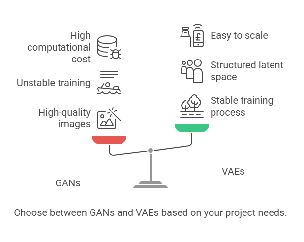
GANs are renowned for their ability to generate highly realistic and sharp images. The adversarial training process encourages the generator to produce outputs that are almost indistinguishable from real data. This makes GANs the preferred choice for applications where visual fidelity is crucial, such as photorealistic image synthesis, deepfakes, and super-resolution.
VAEs:
VAEs, on the other hand, often produce images that are blurrier and less detailed compared to GANs. This is due to the probabilistic nature of their reconstruction process and the regularization imposed by the KL divergence term. However, VAEs excel at capturing the underlying structure of the data and provide a well-organized latent space, which is valuable for tasks like interpolation, clustering, and representation learning.
6.2 Training Stability
GANs:
Training GANs can be notoriously unstable. The adversarial nature of the process often leads to issues such as mode collapse (where the generator produces limited varieties of outputs), vanishing gradients, and oscillating losses. Achieving a balance between the generator and discriminator is challenging and may require careful tuning of hyperparameters, architectural choices, and training strategies.
VAEs:
VAEs are generally more stable and easier to train. The loss function is well-defined and combines reconstruction accuracy with regularization, leading to smoother convergence. While VAEs may not reach the same level of output quality as GANs, their training process is more predictable and less prone to catastrophic failures.
6.3 Practical Considerations
Interpretability and Latent Space:
VAEs provide a structured and continuous latent space, making it easy to explore, interpolate, and manipulate generated data. This is particularly useful for applications like data compression, anomaly detection, and feature extraction. GANs, while powerful, do not inherently provide an interpretable latent space, which can limit their use in certain scenarios.
Flexibility and Extensions:
Both GANs and VAEs have inspired numerous extensions and variants. For example, conditional GANs (cGANs) allow for controlled generation based on labels, while Wasserstein GANs (WGANs) improve training stability. Similarly, conditional VAEs (cVAEs) and β-VAEs offer more control over the generative process and disentanglement of latent factors.
Computational Resources:
GANs often require more computational resources and longer training times due to their adversarial setup. VAEs are typically faster to train and easier to scale to larger datasets.
Python Example: Comparing Outputs
Below is a simple example of how you might compare the outputs of trained GAN and VAE models on the same dataset:
python

def compare_generated_images(generator_gan, decoder_vae, latent_dim, n=10):

    # Generate images from GAN

    noise = np.random.normal(0, 1, (n, latent_dim))

    gan_imgs = generator_gan.predict(noise)

    gan_imgs = gan_imgs.reshape(n, 28, 28)

    # Generate images from VAE

    vae_imgs = decoder_vae.predict(noise)

    vae_imgs = vae_imgs.reshape(n, 28, 28)

    # Plot results

    import matplotlib.pyplot as plt

    plt.figure(figsize=(20, 4))

    for i in range(n):

        # GAN images

        plt.subplot(2, n, i + 1)

        plt.imshow(gan_imgs[i], cmap='gray')

        plt.axis('off')

        if i == 0:

            plt.ylabel('GAN')

        # VAE images

        plt.subplot(2, n, n + i + 1)

        plt.imshow(vae_imgs[i], cmap='gray')

        plt.axis('off')

        if i == 0:

            plt.ylabel('VAE')

    plt.show()
This function allows you to visually compare the quality and characteristics of images generated by both models.
Challenges in Training Generative Models
Training generative models such as GANs and VAEs is a complex process that comes with unique challenges. While these models are powerful, achieving stable and high-quality results often requires addressing specific issues that arise during training. In this section, we’ll discuss common problems like mode collapse in GANs, limitations of VAEs, and practical tips for successful training.
7.1 Mode Collapse and Other GAN Issues
Mode Collapse:
One of the most notorious problems in GAN training is mode collapse. This occurs when the generator starts producing a limited variety of outputs, ignoring the diversity present in the real data. For example, instead of generating a range of handwritten digits, a GAN might only produce images of the digit “3.” This happens because the generator finds a “shortcut” that consistently fools the discriminator, but fails to capture the full data distribution.
Other GAN Challenges:
Training Instability: The adversarial nature of GANs can lead to oscillating losses, vanishing gradients, or the generator and discriminator overpowering each other.
Sensitive Hyperparameters: GANs are highly sensitive to learning rates, batch sizes, and network architectures. Small changes can have a big impact on training dynamics.
Evaluation Difficulty: Unlike supervised models, GANs lack straightforward metrics for evaluating performance. Visual inspection is common, but quantitative metrics like FID or Inception Score are also used.
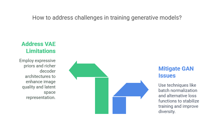
Mitigation Strategies:
Use techniques like batch normalization, label smoothing, and feature matching.
Experiment with alternative loss functions, such as Wasserstein loss (WGAN).
Regularly monitor generated samples and adjust hyperparameters as needed.
7.2 VAE Limitations
Blurry Outputs:
VAEs often generate blurrier images compared to GANs. This is due to the probabilistic reconstruction process and the regularization imposed by the KL divergence term, which can limit the model’s ability to produce sharp details.
Posterior Collapse:
In some cases, the encoder may ignore the latent variables, causing the decoder to generate outputs that do not depend on the latent space. This is known as posterior collapse and can reduce the usefulness of the learned representations.
Limited Expressiveness:
The assumption of a simple prior (usually a standard normal distribution) in the latent space can restrict the model’s ability to capture complex data distributions.
Mitigation Strategies:
Use more expressive priors or hierarchical VAEs.
Adjust the weight of the KL divergence term (e.g., β-VAE).
Employ richer decoder architectures, such as convolutional layers for images.
7.3 Tips for Successful Training
1. Data Preprocessing:
Ensure your data is properly normalized and, if possible, augmented to increase diversity and robustness.
2. Architecture Choices:
Start with simple architectures and gradually increase complexity. For images, convolutional layers often yield better results than fully connected layers.
3. Hyperparameter Tuning:
Systematically experiment with learning rates, batch sizes, and optimizer choices. Use validation data to guide your decisions.
4. Regular Monitoring:
Visualize generated samples and track loss curves throughout training. Early detection of issues like mode collapse or posterior collapse can save time.
5. Use Established Libraries:
Leverage well-tested frameworks and example implementations from libraries like TensorFlow, PyTorch, or Keras. This reduces the risk of implementation errors and provides a solid starting point.
6. Patience and Iteration:
Training generative models can be unpredictable. Be prepared for multiple runs and incremental improvements.
Python Example: Monitoring GAN Training
python

import matplotlib.pyplot as plt

def plot_training_progress(generator, latent_dim, epoch, interval=1000):

    if epoch % interval == 0:

        noise = np.random.normal(0, 1, (10, latent_dim))

        gen_imgs = generator.predict(noise)

        gen_imgs = gen_imgs.reshape(10, 28, 28)

        plt.figure(figsize=(10, 1))

        for i in range(10):

            plt.subplot(1, 10, i+1)

            plt.imshow(gen_imgs[i], cmap='gray')

            plt.axis('off')

        plt.suptitle(f'Epoch {epoch}')

        plt.show()
This function helps you visualize the progress of your GAN during training, making it easier to spot issues early.
Conclusion and Further Resources
Generative models such as GANs and VAEs have transformed the landscape of artificial intelligence, enabling machines to create, imagine, and innovate in ways that were once thought impossible. As we have explored throughout this guide, both models have unique strengths, challenges, and practical applications. In this final section, we’ll summarize the key points, recommend essential libraries and tools, and point you toward further learning resources to deepen your expertise.
8.1 Summary of Key Points
Generative Models: GANs and VAEs are two foundational approaches for generating new data that resembles a training set. GANs use adversarial training to produce highly realistic outputs, while VAEs leverage probabilistic encoding and decoding for structured latent representations.
Implementation: Both models can be implemented in Python using libraries like TensorFlow or PyTorch. While GANs excel at generating sharp, realistic images, VAEs offer stable training and interpretable latent spaces.
Challenges: Training generative models is not trivial. GANs can suffer from mode collapse and instability, while VAEs may produce blurrier outputs and face issues like posterior collapse. Careful architecture design, hyperparameter tuning, and regular monitoring are essential for success.
Applications: These models are widely used in image synthesis, data augmentation, anomaly detection, representation learning, and creative AI applications such as art and music generation.
8.2 Recommended Libraries and Tools
To experiment with and deploy generative models efficiently, consider the following Python libraries and tools:
TensorFlow & Keras: User-friendly APIs for building, training, and deploying deep learning models, including GANs and VAEs.
PyTorch: Flexible and widely adopted deep learning framework, popular in research and production.
NumPy & SciPy: Essential for numerical operations and data manipulation.
Matplotlib & Seaborn: Visualization libraries for monitoring training progress and visualizing generated data.
scikit-learn: Useful for data preprocessing, dimensionality reduction, and evaluation.
Weights & Biases, TensorBoard: Tools for experiment tracking, visualization, and hyperparameter tuning.
8.3 Where to Learn More
The field of generative modeling is rapidly evolving. To stay up to date and deepen your understanding, explore these resources:
Official Documentation:
TensorFlow
PyTorch
Keras
Tutorials and Courses:
Deep Learning Specialization by Andrew Ng (Coursera)
GANs Specialization (Coursera)
Fast.ai Practical Deep Learning for Coders
Books:
Deep Learning by Ian Goodfellow, Yoshua Bengio, and Aaron Courville
Generative Deep Learning by David Foster
Research Papers:
Generative Adversarial Nets (Goodfellow et al., 2014)
Auto-Encoding Variational Bayes (Kingma & Welling, 2013)
Open Source Implementations:
Keras GAN Examples
PyTorch VAE Example
Community and Forums:
Engage with the AI community on platforms like Stack Overflow, Reddit r/MachineLearning, and Kaggle to ask questions, share projects, and learn from others.
AI Agents in Practice: How to Automate a Programmer’s Daily Work
Building AI Agents: A Practical Approach to Python
Ethical Challenges in Artificial Intelligence Development: What Should an AI Engineer Know?